I came across this paper “Implicit Rank-Minimizing Autoencoder” [1] by FAIR which was shared by Yann LeCun on his facebook timeline. In this paper, the authors show that inserting a few linear layers between the encoder and the decoder decreases the dimensionality of the latent space. The authors build on the results of [2] which showed how overparameterization of linear neural networks results in implicit regularization of the rank when trained via gradient descent(GD). I will summarize some previous works related to implicit regularization with GD and then discuss the results of this paper.
Optimizing linear neural networks via gradient descent leads to low rank solutions.
This has been well studied in the past in the context of matrix factorization in Gunasekar[3] and Arora[4]
First, let us get an intuition of how gradient descent brings implicit regularization in overparameterized setting. Imagine if we have simple least squares problem. So our loss function is $L(\textbf{w}) = \frac{1}{2}||X\textbf{w} - Y||^2$. There exists closed form solutions for this but let us see how optimizing this via gradient descent is. This is what the learning dynamics would look like.
$$\textbf{w}^{(t+1)} = \textbf{w}^{(t)} - \eta\nabla_{\textbf{w}} \quad\quad\quad (1)$$where $\nabla{\textbf{w}} = \nabla_{\textbf{w}}L(\textbf{w})$ (Omitting $L(\textbf{w})$ for brevity)
Note that if we add another parameter, a scalar $w$, i.e, $\textbf{w} = \textbf{w}_1w_2$, we do not change the representational capacity because of linearity. So replacing that and taking the derivative of $L(\textbf{w}_1,w_2)$ w.r.t $\textbf{w}_1$ and $w_2$, we notice that the gradient descent update for $\textbf{w}=\textbf{w}_1w_2$ would look like
$$\textbf{w}^{(t+1)} = (\textbf{w}_1^{(t)} - \eta\nabla_{\textbf{w}_1})(w_2^{(t)} - \eta\nabla_{w_2})$$ $$= \textbf{w}_1^{(t)}w_2^{(t)} - \eta w_2^{(t)} \nabla_{\textbf{w}_1^{(t)}} - {\eta \nabla _{w^{( t)}_{2}}\mathbf{w}^{( t)}_{1}} + { O \left( \eta ^{2}\right)}$$ $$= \textbf{w}_1^{(t)}w_2^{(t)} - \eta (w_2^{(t)})^2 \nabla_{\textbf{w}^{(t)}} - {\eta (w_2^{(t)})^{-1} \nabla _{w^{( t)}_{2}}\mathbf{w}^{(t)}} + { O \left( \eta ^{2}\right)}$$ $$\implies \textbf{w}^{(t+1)} = \textbf{w}^{(t)} - \rho^{(t)} \nabla_{\textbf{w}^{(t)}} - {\gamma^{(t)} \mathbf{w}^{(t)}} \quad\quad\quad (2)$$
Note that we have used $\nabla \mathbf{_{w_{1}}} L(\mathbf{w}_{1} ,w_{2}) \ =\ \frac{\partial ( L(\mathbf{w}_{1} ,w_{2}))}{\partial \mathbf{w}}\frac{\partial (\mathbf{w})}{\partial \mathbf{w}_{1}} \ =\nabla _{\mathbf{w}}\frac{\partial (\mathbf{w}_{1} w_{2})}{\partial \mathbf{w}_{1}} \ =\nabla _{\mathbf{w}} w_{2}$
and set $\rho^{(t)} = \eta (w_2^{(t)})^2$ and ${\gamma^{(t)}} = \eta (w_2^{(t)})^{-1}\nabla _{w^{( t)}_{2}}$ and neglected the $O(\eta^2)$ terms because $\eta$ is usually very small.
See that $(2)$ looks similar to $(1)$ except for another additive factor. And each $\mathbf{w}^{(t)}$ contains a part of $\nabla_{\textbf{w}}$ which shows that this is nothing but the momentum term that we are familiar with. We see that overparameterizing by one scalar term implicitly changes the learning dynamics by manifesting as the momentum term. The above derivation is given in full detail as Observation 1 in [4]
[2] then considers a linear neural network where there are N linear layers with no non-linearlity between them. Functionally, it is equivalent to
$$W_e = W_NW_{N-1}...W_1 \quad\quad\quad (3)$$where $W_i$ represent the weights of the layers and $W_e$ is the overall end-to-end effective weight. Note that by doing this, there is no change in the representational capacity of the neural network(again due to linearity), we are only overparameterizing by adding linear layers to see how it affects the learning dynamics.
[2] showed that for a linear layer network represented by $(3)$ the singular values of the same follow the learning dynamics given by
$$\sigma_r(t + 1) = \sigma_r(t) - \eta \cdot \langle \nabla L(W(t)) , \mathbf{u}_r(t) \mathbf{v}_r^\top(t) \rangle \cdot {N \cdot (\sigma_r(t))^{2 - 2 / N}} \quad\quad\quad (4)$$Putting $N=1$, we recover the case of $W_e = W_1$ (i.e no overparameterization) and we notice that $(4)$ becomes
$$\sigma_r(t + 1) = \sigma_r(t) - \eta \cdot \langle \nabla L(W(t)) , \mathbf{u}_r(t) \mathbf{v}_r^\top(t) \rangle \quad\quad\quad (5)$$Comparing $(4)$ with $(5)$, we note that by overparameterization of $W$ in gradient descent, the singular values of $W$ are regularized by the additonal multiplicative factors $N$ and $(\sigma_r(t))^{2 - 2 / N}$ . While $N$ is constant for all singular values, $(\sigma_r(t))^{2 - 2 / N}$ has more effect on larger $\sigma_r(t)$ and less on smaller $\sigma_r(t)$. Also note that $(3)$ doesn’t depend on width of the linear layers so
$$W_e = W_Nw_{N-1}...w_2W_1 $$where $w_i, i = N-1$ to $2$ are scalars achieves the same regularization effect on the singular values of $W_e$.
The complete proof of $(4)$ is given in Section B.4 of [2]. The proof requires the use of another theorem stated below
$$W(t+1) \leftarrow W(t) - \eta \cdot \sum\nolimits_{j=1}^{N} \left[ W(t) W^\top(t) \right]^\frac{j-1}{N} \nabla{L}(W(t)) \left[ W^\top(t) W(t) \right]^\frac{N-j}{N} $$This holds true under certain assumptions on the initialization of $W$ which is usually true. The proof of $(5)$ is given in Section A.1 of [4]. It’s worth going through the proof to really convince yourself.
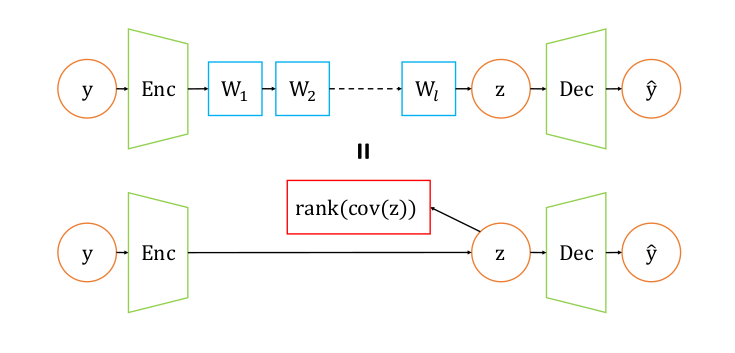
And thus we have seen how minimizing an overparameterized $W$ (Linear Neural Networks) via gradient descent leads to low-rank solutions. This fact is used in [1] to implicitly reduce the dimensions of the latent space by inserting a few linear layers after the encoder. Those linear layers produce a low-rank latent space governed by $(2)$. The authors call their autoencoder “IRMAE” and perform a number of tests to validate the theoretical analysis.
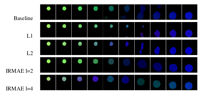
In the first section, they create a toy dataset of images containing either a square or circle filled with a colour centered at random coordinates and compare the results of a standard autoencoder vs their proposed IRMAE. Implicitly, this task has a dimension of 7 (3 for each of RGB, 2 for coordinates(x and y) and 2 for shape(square or circle)). They show that IRMAE with $l=2$ is able to achieve this theoretical rank as compared to the standard AE. $l$ refers to the number of linear layers after the encoder.
They also show the results obtained in MNIST and CelebA dataset which highlights the improved performances of IRMAE over standard AE. I implemented it on the MNIST dataset and was able to reproduce the results shown in the paper. And the latent space learned by IRMAE produces much higher quality images than the standard AE. Even the interpolation is smoother and of higher quality.
Ablation studies are performed to verify that the reduction in dimension of generated latent space happens due to implicit regularization of GD and not due to influence of other factors. The three ablation studies performed were :-
-
Fixed - All the linear layers have their weights frozen. The result of this is a weakened regularization effect and worsening of the quality of generated samples. This shows that the dimension reduction is not due to just the architecture.
-
Non Linearity - The linear layers now have non linearity between them which is equivalent to a deeper encoder architecture. This regularization effect was not present at all. This indicates that it is also not due to deeper architecture.
-
Weight Share - All the linear layers share the same weights. The result of this is also a weakened regularization effect.
The results of the above studies show that the dimensionality reduction is due to the learning dynamics on the over-parameterized setting of the weight matrix which is consistent with the theoretical analysis.
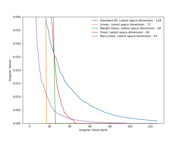
I used Google Colab to reproduce only the results on the MNIST dataset and below is the trimmed plot of singular values of the latent space’s covariance matrix evaluated on the test dataset. I was able to reproduce the results mentioned in the paper. The learned latent space by IRMAE has much lower dimensionality than the latent space learned by a standard AE.
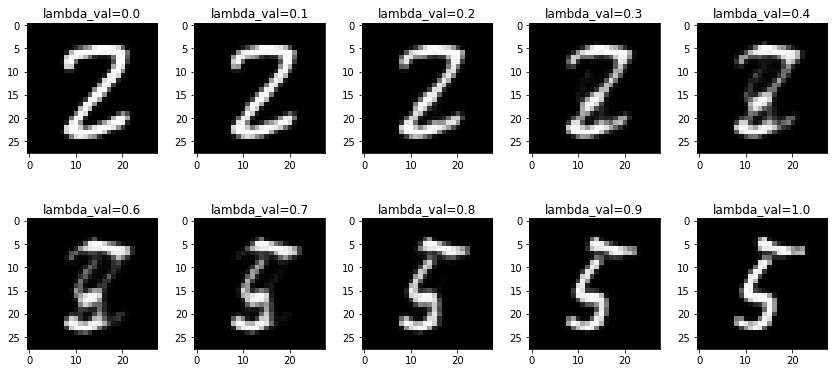
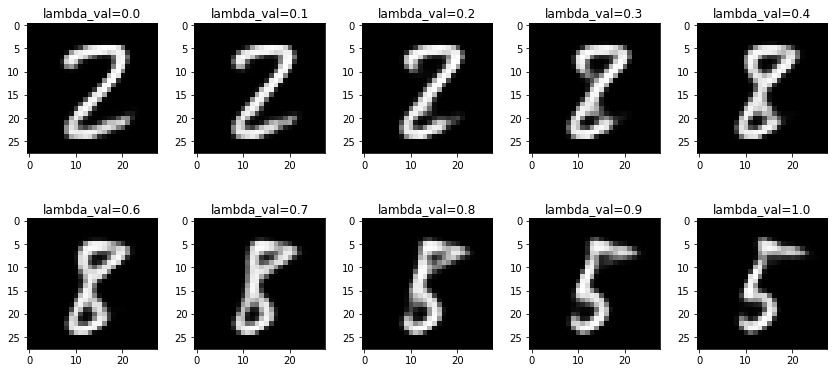
And I tested the interpolation results which are much better than the standard AE as expected. The learned latent space in a standard AE is not rich and expressive like the one learned by a Variational AE which models the latent space as a distribution. But since IRMAE learns a low-rank latent space, we can expect it to have modelled the lower dimensional manifold in which the data exist. And interpolation in a standard AE produces many artifacts when $\lambda$ is around 0.5 unlike IRMAE as is evident from the comparisons.
The code for the above results is here. I used this as a reference for the standard autoencoder and built on top of it to add the linear neural network after the encoder.
This was an interesting read and I have been exploring other papers in this direction. A lot has yet to be understood by the generalization phenomenon exhibited by gradient descent. Another very recent paper shows that GD tries to penalize trajectories that have large loss gradients and steer the descent towards flatter loss regions where the test errors are low and is more robust to parameter pertubations. They employ backward error analysis to calculate the size of this implicit regularization as well.
Hope this post helped understand some basic aspects of implicit regularization by gradient descent. Do read the IRMAE[1] paper, they analyse the results in more detail and it’s easy to follow and insightful.
*Fig are figures directly taken from the IRMAE paper
References:
- [1] Li Jing, Jure Zbontar, Yann LeCun Implicit Rank-Minimizing Autoencoder
- [2] Sanjeev Arora, Nadav Cohen, Wei Hu, Yuping Luo Implicit Regularization in Deep Matrix Factorization
- [3] Suriya Gunasekar, Blake Woodworth, Srinadh Bhojanapalli, Behnam Neyshabur, Nathan Srebro Implicit Regularization in Matrix Factorization
- [4] Sanjeev Arora, Nadav Cohen, Elad Hazan On the Optimization of Deep Networks: Implicit Acceleration by Overparameterization
- Can increasing depth serve to accelerate optimization?
- Understanding implicit regularization in deep learning by analyzing trajectories of gradient descent