It took me forever to understand what Gaussian Processes(GPs) were all about. I have been trying to understand it for quite some time but always gave up after the initial hurdle. And I think it happened because I got confused by the way a Gaussian Process is portrayed that I came across in many blog posts.
The introductory text on GPs usually talk about how it can be used to model arbitrary smooth functions non-parametrically. And to set up a GP, you need to define the covariance matrix of a multivariate gaussian. And to populate that matrix, one needs to evaluate the kernel function that forms the basis of a GP. As I was trying to understand this, all I could think was, how would this be able to generate smooth functions as the plots show them to be? To plot a function in a smooth manner, one needs to know the equation of the curve(the parameters of a family of curves). But that is exactly what GPs avoid. We do not want to learn the parameters of the curve. Instead, how do we non parametrically model the data? And this left me scratching my head for a good while until it finally clicked.
Turns out, as expected, there was a gap in my thought process. The graphs that I was observing, the ones that show random samples from a GP, weren’t actually plots of smooth functions even though they appear to be smooth. That’s because usually when plotting a set of points of a curve, it is usually shown as a smooth curve by default. This isn’t something I didn’t know, but somehow, this never clicked while I was observing those plots. That is, until recently when I approached the topic with a fresh mind.
In a GP, we try to model the train and test output data points jointly as a multivariate Gaussian random variable. To define a multivariate gaussian, we need to define the mean of each component and the covariance matrix that encodes how each of those components behave with respect to each other. The detail lies in how the covariance matrix is defined.
Let’s take an example to illustrate. Imagine there is a function $f$ that produces an output $y$ given the input $x$, i.e, $y = f(x)$. Now let’s say one has observed a few points, $x_{1...N}$ and their outputs $y_{1...N}$. GPs help us model this function $f$ non-parametrically so that we can find the output of previously unseen input points, without having to learn any parameters. Let’s now say that we want to evaluate the model on $M$ new inputs, i.e, $x{^*}_{1...M}$ to get the outputs $y{^*}_{1...M}$.
The way this is done in a GP is to assume that the collection of output variables, both test and train, are jointly distributed according to a Gaussian distribution.
$$ \begin{bmatrix} y_1 \\ y_2 \\ ... \\ y_N \\ y{^*}_{1} \\ y{^*}_{2} \\ ... \\ y{^*}_{M} \\ \end{bmatrix} \sim N(\begin{bmatrix} 0 \\ 0 \\ ... \\ 0 \\ \end{bmatrix}, K) $$And the covariance matrix is defined as follows.
$$ K = \begin{bmatrix} k(x_1, x_1) \hspace{1em} k(x_1, x_2) \hspace{1em} ... \hspace{1em} k(x_1, x_N) \hspace{1em} k(x_1, x{^*}_1) \hspace{1em} ... \hspace{1em} k(x_1, x{^*}_M) \\[1em] k(x_2, x_1) \hspace{1em} k(x_2, x_2) \hspace{1em} ... \hspace{1em} k(x_2, x_N) \hspace{1em} k(x_2, x{^*}_1) \hspace{1em} ... \hspace{1em} k(x_2, x{^*}_M) \\[1em] ... \\[1em] k(x_N, x_1) \hspace{1em} k(x_N, x_2) \hspace{1em} ... \hspace{1em} k(x_N, x_N) \hspace{1em} k(x_N, x{^*}_1) \hspace{1em} ... \hspace{1em} k(x_N, x{^*}_M) \\[1em] k(x{^*}_1, x_1) \hspace{1em} k(x{^*}_1, x_2) \hspace{1em} ... \hspace{1em} k(x{^*}_1, x_N) \hspace{1em} k(x{^*}_1, x{^*}_1) \hspace{1em} ... \hspace{1em} k(x{^*}_1, x{^*}_M) \\[1em] ... \\[1em] k(x{^*}_M, x_1) \hspace{1em} k(x{^*}_M, x_2) \hspace{1em} ... \hspace{1em} k(x{^*}_M, x_N) \hspace{1em} k(x{^*}_M, x{^*}_1) \hspace{1em} ... \hspace{1em} k(x{^*}_M, x{^*}_M) \\[1em] \end{bmatrix} $$is a $(N+M)$ x $(N+M)$ matrix, where $k$ is called the kernel function, whose purpose is to indicate how the outputs of different $x_i$’s and $x_j$’s are correlated with each other. Note the entries of the matrix which are the evaluation of the kernel function for all pairs of input points, both train and test.
Essentially, if I know that the outputs of $x_i$ & $x_j$ are highly correlated(which is given to us by computing the kernel function), then I can guess $y_j$ if I know what $y_i$ is. So, now you can imagine, in a smooth function, the function changes very gradually around any point. To capture this in a GP, we want the kernel function to give higher correlation value for points closer together and lower for points that are farther apart. Note: This is just one of the behaviours, there are other kernel functions that capture different kinds of behaviour like periodicity. The takeaway is that the kernel function, which is used to compute the covariance matrix of the joint distribution, defines the kind of functions the GP can model. We’ll see a few examples later.
So by knowing how the outputs are correlated with each other, one can condition the unobserved outputs $y^*$ against the observed ones $y$ and sample from the Gaussian random variable for possible values of $y^*$.
A brief refresher on conditional gaussian random variables is as follows. A bivariate Gaussian is represented as
$$ \begin{bmatrix} A \\ B \\ \end{bmatrix} \sim N(\begin{bmatrix} \mu_{A} \\ \mu_{B} \\ \end{bmatrix}, \begin{bmatrix} K_{AA} \ K_{AB} \\ K_{BA} \ K_{BB} \\ \end{bmatrix} ) $$where A and B are two components. Note that A and B can both represent subsets of multiple components and the random variable will be a multivariate gaussian.
An important feature of the Gaussian is that conditioning a set of its variables against the remaining set, still behaves as a Gaussian whose mean and covariance matrix can be computed from the conditioning variables. So
$$ B|A \sim N(\mu_{B|A}, K_{B|A}) $$where
$$ \mu_{B|A} = \mu_{B} + K_{BA}K_{AA}{^{-1}}(A - \mu_{A}) \tag{1} $$and
$$ K_{B|A} = K_{BB} - K_{BA}K_{AA}{^{-1}}K_{AB} \tag{2} $$What this tells us is, if we have already observed the value of $A$, we can condition $B$ on $A$, to get the conditional distribution of $B|A$ from the joint distribution of $A,B$. And this is the principle on the basis of which GPs work. They are also referred to as uncertainty models, because they quantify the uncertainty of unobserved input space. We’ll see later how we can quantify uncertainty ranges.
Now it should be clear how we can sample from the conditional gaussian to get values for the unobserved data points.
Let $Y$ represent $y_{1...N}$, the observed outputs, and $Y^*$ represent $y{^*}_{1...M}$, the unobserved outputs. And $X$ and $X^*$ represent the respective observed and unobserved inputs.
$$ \begin{bmatrix} Y \\ Y{^*} \\ \end{bmatrix} = \begin{bmatrix} y_1 \\ ... \\ y_N \\ y{^*}_{1} \\ ... \\ y{^*}_{M} \\ \end{bmatrix} \sim N(\begin{bmatrix} 0 \\ 0 \\ ... \\ 0 \\ \end{bmatrix}, K) \tag{3} $$Then, from above discussions about conditional gaussian distribution, we can write
$$ Y*|Y,X,X* \sim N(\mu_{Y^*|Y}, K_{X^*|X}) $$This is also called the posterior distribution, i.e, the distribution of the test outputs after observing the train data.
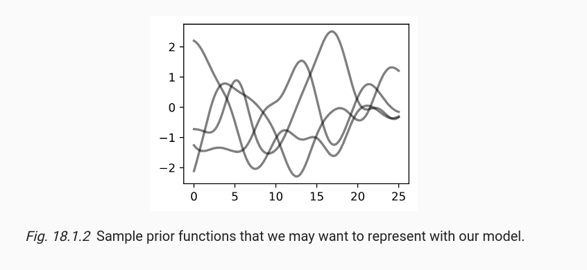
The following figure shows random samples of a GPs. Which is basically the prior distribution, when we do not have any knowledge of the function at the train points. These points are sampled from the prior distribution :-
$$ Y*,Y|X,X* \sim N(\mu_{(Y^*,Y)}, K_{(X^*,X)}) $$This is the same as Eqn $(3)$.
The plot above shows three randomly sampled “functions” from a certain GP. I write functions in quote because, as I had mentioned in the beginning, this is not actually a function being sampled, but points being sampled from a multivariate gaussian. And the points are connected smoothly while plotting to depict a randomly sampled “function” from a GP.
The procedure to initialize a GP is as follows :-
- Decide on the input space and create a grid of train and test input points. (In the above example plot, the grid is a collection of 25 linearly spaced points in the interval $[-10, 10]$ on the X-axis).
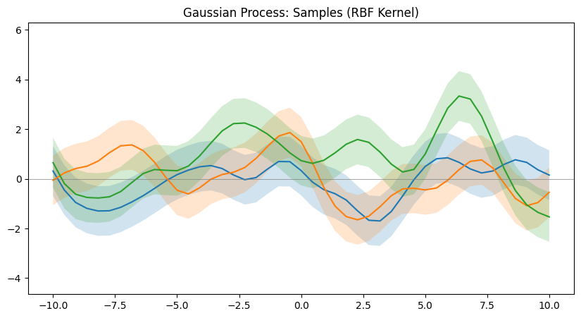
- Choose a valid kernel function $k$ to compute the covariance matrix of the joint distribution. The kernel decides what kind of functions the GP can model. Some examples include :-
- Radial Basis Function kernel
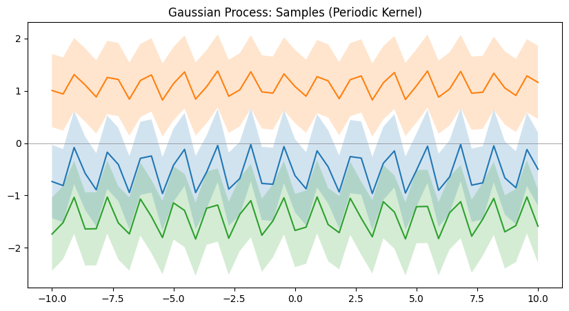
- Periodic kernel
- Linear kernel
- Define a multivariate gaussian with N components, whose mean can be assumed to be $0$ vector and the covariance matrix as computed from the kernel using the grid of input points.
Now sampling once from this multivariate gaussian will give you one set of N points that is basically the function that we see in the plot. In the above example plot, you see 25 points of three such functions sampled and plotted. This gives an idea about what kind of function the kernel can help model.
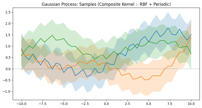
Different kernels are able to represent different kinds of function. And more complex kernels can be created by combining simple kernels together. Below are a few examples of such kernels.
Now that we understand how GPs are able to model relationships, we can proceed to see an example of how we can use one to guess the outputs of test data points after seeing a few training data points. And as mentioned before, GPs are also able to quantify the uncertainty at different regions, so we can visually see how uncertain the model is at different regions of the input domain. This is equivalent to observing the standard deviation of the GP at a certain point and drawing a $[-\sigma,+\sigma]$ range of shaded regions around the point to visually see it. And another useful property of Bayesian optimization(in which GPs are commonly used) is that, we can also have an idea about what input points should the model observe the outputs of next so that it can reduce the uncertainty where it is high. This is helpful when it is expensive to evaluate the function we are trying to model.
Here in the following example, an RBF Kernel GP is being trained to model a random polynomial function:-
$$ y = x^3 + 4x^2 + x - 1 $$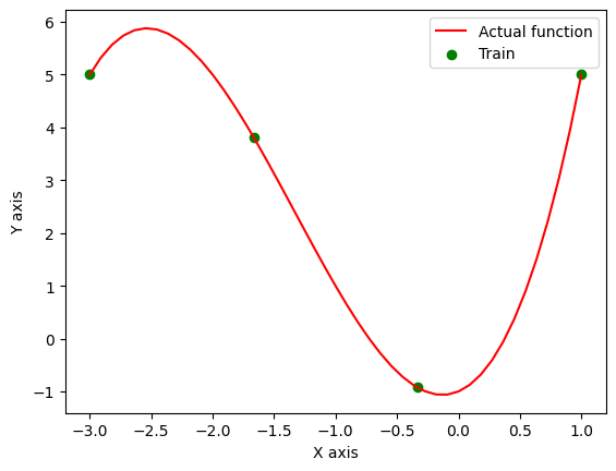
Only 4 observations to be used for GP. And here is what the GP is able to predict for the other points in the region.
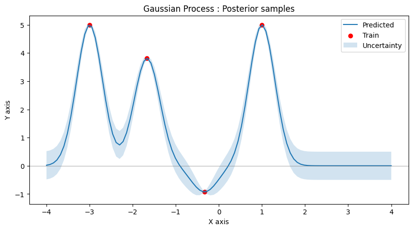
Notice how the uncertainty varies in the input space, lower at observed areas and higher otherwise.
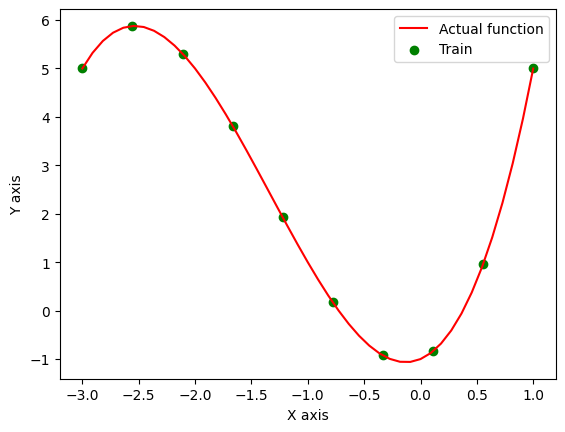
Let’s see how the uncertainty of the model changes upon observing 10 points instead.
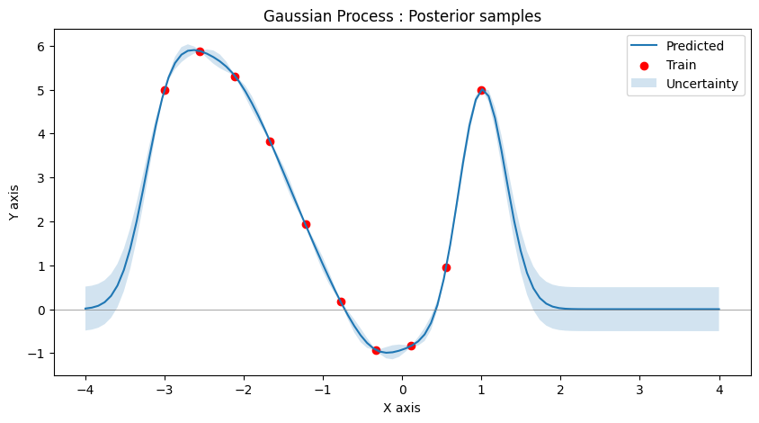
It is clear that the model is now less uncertain at the points where new observations has taken place as compared to other regions.
GPs are advantageous because uncertainty is an intrinsic part of the model. And the usage of kernel function brings all the good properties of kernel methods along with it. But a vanilla GP is not very scalable, since we need to invert a matrix which scales as $O(n^3)$ which becomes unusable for analysing a large input region. And the vanilla form of GP outputs only scalar values. Extending this to multi-dimensions is quite involved and there are several ways to do it. Many frameworks have been written focussing on GPs like GPytorch, etc. Worth looking if one is interested in practical usage.
The roughly written code used for this blog post can be found at this link :- dibyadas/gaussian_processes
The important part of the code to focus on is the following :-
def posterior_samples(self, train_X, train_Y, N=25):

        train_X = np.array(train_X)
        train_Y = np.array(train_Y)

        # get the grid of input points
        start, stop = self.interval
        points = np.linspace(start, stop, N)

        # calculate the covariance matrix, i.e, the K matrix of all possible pairs of input points
        cov = [[self.kernel(x,y) for y in train_X] for x in train_X]

        # Below, A refers to train points and B refers to test points

        # function to compute K_BA matrix, which is the same as K_AB
        k_vector = lambda new_point : np.array([self.kernel(point, new_point) for point in train_X])

        # function to compute K_BB matrix
        c = lambda new_point : self.kernel(new_point, new_point)

        # inverse of K_AA matrix
        cov_inv = np.linalg.inv(cov)

        # implementation of Eqn (1)
        predicted_mean = lambda new_point : k_vector(new_point).T @ cov_inv @ train_Y

        # implementation of Eqn (2)
        predicted_var = lambda new_point : c(new_point) - k_vector(new_point).T @ cov_inv @ k_vector(new_point)

        predicted_means = np.array([predicted_mean(point) for point in points])
        predicted_vars = np.array([predicted_var(point) for point in points])
This just barely scratches the surface of Gaussian Processes. There are a few resources which I read that I want to highlight because they were clear and rich in their explanations. This blog post from distill.pub is a great starting reference article and even has interactive plots to help understand GPs. This blog post from Ludwig Winkler introduced me to the idea of adding information about derivatives of the function. Which adds to the information we can use to improve our guess about the unobserved variables leading to more accurate/useful GPs. Their other blogs are also worth a read. This youtube video from Mutual Information visually explains the fundamentals.
Sometimes it’s okay to get confused by a concept intially. Because it indicates that there might be something more fundamental to understand before it.