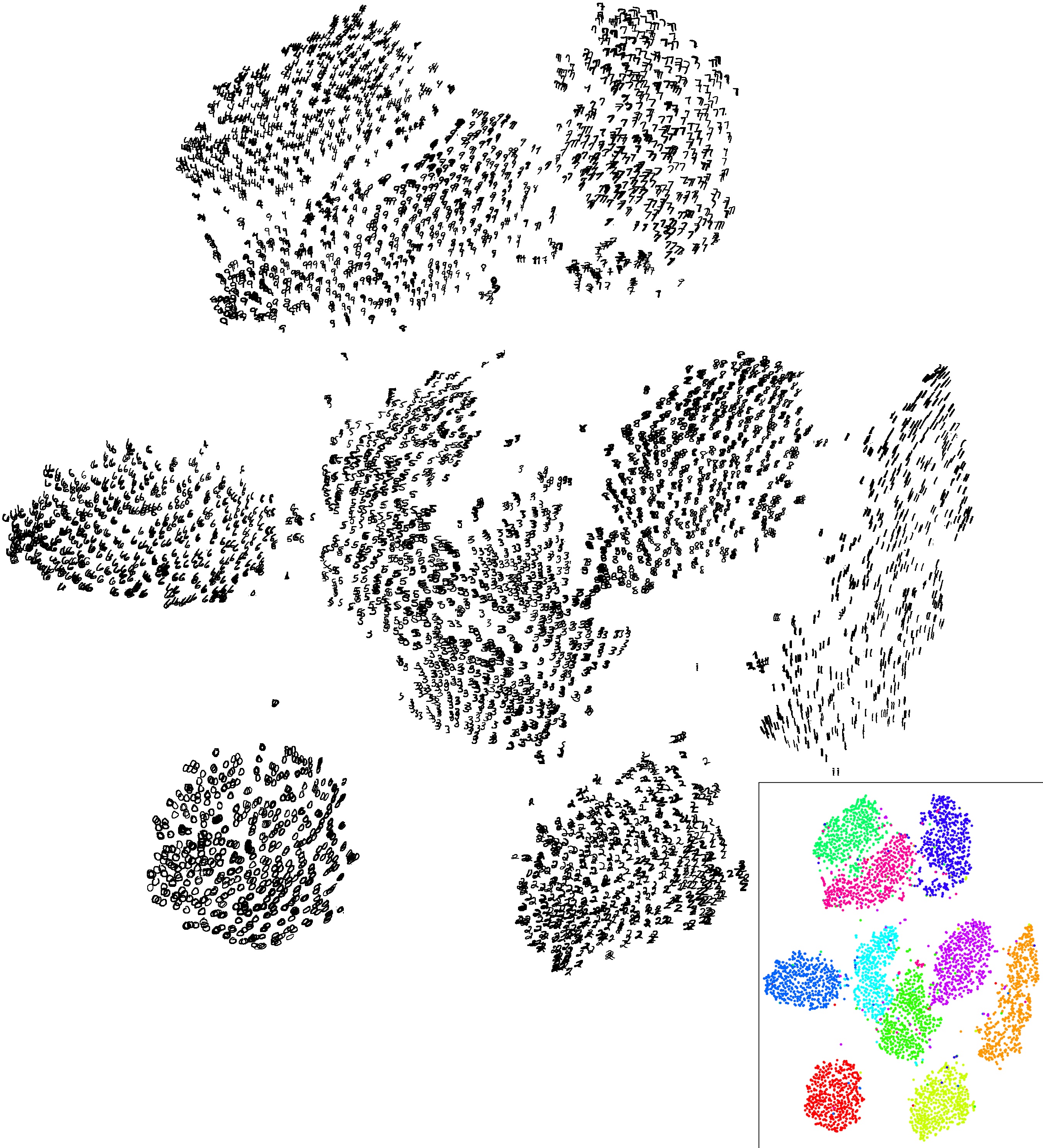
I first heard about t-SNE a few years back as tool to help visualize high-dimensional data in 2D or 3D. And I had come across these amazing visualizations which displayed MNIST dataset in a 2D map which immediately drew my attention. Another one I came across which showed the different clusters of Fashion MNIST data in 3D. I didn’t think of it much until very recently when I thought of reading the details of what t-SNE is and how it works.
I read the original paper of t-SNE which was published in 2008. The paper is clearly written and I could understand what the authors were trying to do.
Visualizing high dimensional data is tricky, because you are bound to lose some information when you are projecting down to 2D/3D, and so the distances between points can’t be perfectly preserved. A well known simple technique for dimensionality reduction is PCA. We can select the first 2 or 3 principal components which retain the maximum information and we use that to display the data points in a 2D/3D space. While it’s easy to understand and reason about, it does not work well on non-linear data. For instance, a low-dimensional non-linear surface embedded in a high-dimesional space will be difficult to analyze using PCA. This is because PCA cannot understand any non-linear dependencies among the features. So is there a way to represent global and local structure of a high-dimensional data when visualizing in 2D/3D? Yes there is. There are many different ways and t-SNE is one of them which we’ll understand in this blog post. These fall under the category of non-linear dimensionality reduction techniques whose aim is to capture meaningful relationship among points in a high-dimensional space to faithfully represent those relations in lower dimension.
Now let’s dive into the subject of this post. We’ll go along according to the paper. The SNE in t-SNE stands for Stochastic Neighbour Embedding. SNE is a general technique and t-SNE is one enhancement of it. The core idea is to define a conditional probability distribution for each point in the high-dimensional data. Let there be $N$ data points $X_{1...N}$ and the probability distribution is defined for each point of the data set. $p_{j|i}$ is defined as the probabilty that $x_i$ will select $x_j$ as its neighbour. Naturally, we want this to be higher for points that are closer together and lower for points that are farther apart. This conditional distribution aims to capture the local structure of the data. Let this distribution on data points be denoted as $P$. The next step is to generate $N$ random low-dimensional points $Y_{1...N}$ called as map points. Now a similar construction of probability distribution can be done on the map points. Let the distribution on map points be denoted as $Q$. The goal is to make $Q$ similar to $P$ such that the map points are able to capture this neighbourhood relationship amongst each other as it is with the original data points. The metric used to capture the error between two probability distrubtions $P$ and $Q$ is the KL divergence metric from $P$ to $Q$.
The distribution $p_{j|i}$ is defined using a Gaussian kernel :-
$$ p_{j|i} = \frac{exp(- ||x_i - x_j||^2 / 2\sigma^2_i)}{ \sum_{k \not= i} exp(- ||x_i - x_k||^2 / 2\sigma^2_i)} $$What this represents is, the probability that the data point $x_i$ will select another data point $x_j$ as its neighbour is equal to the value of a Gaussian distribution at $x_j$ if it is centered on $x_i$ with an appropiately set variance $\sigma^2_i$. And $p_{i|i}$ is a trivial fact and is set to 0 to not waste probability mass on it. A similar construction can be done for the corresponding map points by defining a distribution
$$ q_{j|i} = \frac{exp(- ||y_i - y_j||^2 )}{ \sum_{k \not= i} exp(- ||y_i - y_k||^2 )} $$for each point $y_i$. Note that the $\sigma_i^2$ is set to $\frac{1}{\sqrt 2}$ for every map point. Which suggests that the map points aren’t a perfect model for the data. For example, even if we try to map a 2D bimodal gaussian mixture of two different densities to another 2D space, the varying densities might be hard to observe. Both the clusters might appear equally dense which is not the case. In other words, local densities of data points is not explicitly assumed in the map points and any observed densities is due to the pushing and pulling of the points with respect to each other as we adjust map points so that $Q$ resembles $P$.
And the cost function for this problem is KL divergence, which is not symmetric. This causes different deviations to be weighted differently. For this problem, it is defined as :-
$$ C = KL(P|Q) = \sum_{i=1}^{N} KL(P_i|Q_i) = \sum_{i=1}^{N} \sum_{j=1}^{N} p_{j|i} \log\frac{p_{j|i}}{q_{j|i}} $$There is a larger penalty if $p_{j|i}$ is large and the correspoing map points represent a small $q_{j|i}$, which is, that nearby data points $x_i$ and $x_j$ are being represented by far away map points $y_i$ and $y_j$. And a smaller penalty when $p_{j|i}$ is small and $q_{j|i}$ is large, i.e, far away data points are being represented by nearby map points. The gradient of the cost function with respect to the map points, for this particular setup, can be analytically derived and understood as points being joined by springs which are pushing/pulling on each other and the forces on the springs are governed by how close the corresponding data points are in the high-dimensional space. The paper has a good explanation of this idea and it is worth checking out. The cost function emphasizes majorly on ensuring that nearby data points are represented by nearby map points.
The other thing to note is that, each of the $p_{j|i}$ has a $\sigma^2_i$ to be defined. The $\sigma^2_i$ is the size of the Gaussian kernel of that point. This corresponds to deciding how many neighbours each point should have. Naturally, points with many nearby points(dense regions) should have a smaller size whereas points without as many nearby points should have a larger size, so that there effective number of neighbours would roughly be the same. This is referred to as the Perplexity for the SNE problem which is user-specified. It is defined as :-
$$ Perp(P_i)=2^{H(P_i)} $$$$ H(P_i) = - \sum_{j}p_{j|i}\log_2 p_{j|i} $$
where H is the usual entropy function of a probability distribution. So for every $P_i$ an appropiate $\sigma_i$ is found so that all of the $P_i$’s have the same perplexity(equivalently, the same entropy). This is done once for a data set and, in the paper implementation, binary search is used to find the appropiate $\sigma_i$’s for each $x_i$. Here is an interactive plot you can use to observe how, for the same perplexity value, different points have different radius of the kernel.
The authors then give a momentum based gradient descent algorithm formula to arrange the map points. They also point out few tricks like simulated annealing, which is adding decreasing levels of noise during the training part to ensure the points get large forces to move away from each other in the beginning and settle on a structure by the end of the training.
The paper then highlights a problem that SNE suffers from. The crowding problem. It refers to the fact that we cannot preserve all distances in the high-dimensional dataset in low dimension and we are bound to place some nearby data points farther then they should be compared to other points but there is not enough “space” to do so. Below is a figure I drew to understand the crowding problem.
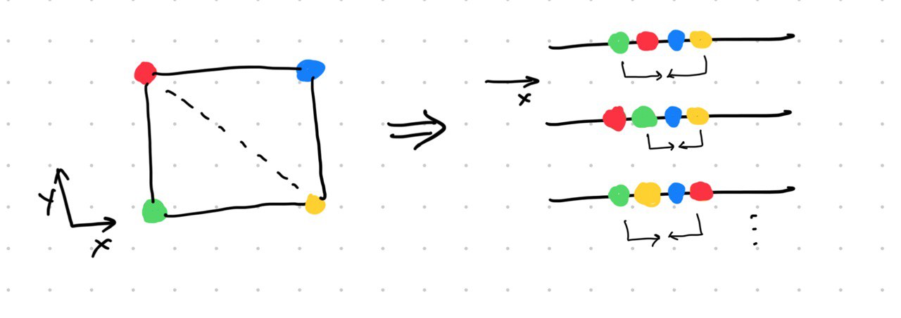
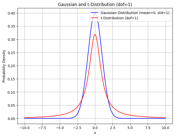
No matter how we map those 2D points on a line, we will always have a situation where one point is placed too far as compared to another even though both points might be equally nearby in the 2D space. On the right hand side, in the first mapping, the red point’s neighbours are represented well but the yellow point is too far away from the green point even though green is as close to red as it is to yellow in the original space. This results in some attractive force between the points. Mathematically, it is when $p_{j|i}$ is small but not neglectable and $q_{j|i}$ is too small. This results in some attractive forces on the map points which corresponds to the data points from different clusters to have some attractive forces amongst themselves and be pulled close together and thereby reducing the visual distinction between the clusters. To solve this problem, the authors propose a variant of SNE called t-SNE which uses a Student’s t distribution with 1 degree of freedom to model the map points instead of a Gaussian. t-distribution has heavier tails than a Gaussian, and what this allows is, some room for error for the map points which are representing nearby points by increasing the value of $q_{j|i}$. So now the attractive forces are relaxed because the difference between it and $p_{j|i}$ is lesser as compared to when using a gaussian. Deepfindr explained this very well on their video.
The additional benefit this brings is that it is now easier to calculate the gradients of the cost function, as the exponentiation is no longer required. The $q_{j|i}$ is now given by :-
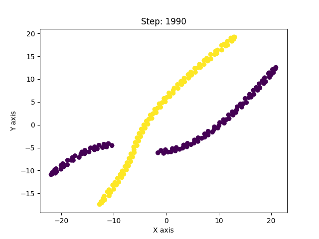
$$ q_{j|i} = \frac{(1 + ||y_i - y_j||^2 )^{-1}}{ \sum_{k \not= i} (1 + ||y_i - y_k||^2 )^{-1}} $$I referred to the official implementation of t-SNE in Python and ran a few experiments. First, I generated points from two 3D helices separted by a phase which can be seen below.
I have also shown how PCA is unable to separate out the two "cluster"s of points. Now, I ran the original t-SNE implementation and below is a GIF of how the map points evolved to form two separate clusters of data.
Notice how after the 100th step, the local structure takes precedence since the early exaggeration is stopped
(Have only shown 200 iterations as this converged pretty quickly)
The implementation is simple and it is worth the effort to go through it.
def tsne(X=np.array([]), no_dims=2, initial_dims=50, perplexity=30.0):
    """
        Runs t-SNE on the dataset in the NxD array X to reduce its
        dimensionality to no_dims dimensions. The syntaxis of the function is
        `Y = tsne.tsne(X, no_dims, perplexity), where X is an NxD NumPy array.
    """

    # Check inputs
    if isinstance(no_dims, float):
        print("Error: array X should have type float.")
        return -1
    if round(no_dims) != no_dims:
        print("Error: number of dimensions should be an integer.")
        return -1

    # Initialize variables
    X = pca(X, initial_dims).real
    (n, d) = X.shape
The first step t-SNE performs is PCA to convert the high dimensional data into a somewhat lower dimensional space but not too low. The default value is set to 50.
    max_iter = 1000
    initial_momentum = 0.5
    final_momentum = 0.8
    eta = 500
    min_gain = 0.01
    Y = np.random.randn(n, no_dims)
    dY = np.zeros((n, no_dims))
    iY = np.zeros((n, no_dims))
    gains = np.ones((n, no_dims))
A few parameters intialization happens then. The learning rate, timesteps, momentum weights and so on.
    # Compute P-values
    P = x2p(X, 1e-5, perplexity)
    P = P + np.transpose(P)
    P = P / np.sum(P)
    P = P * 4.									# early exaggeration
    P = np.maximum(P, 1e-12)
Here the $P$ matrix is initialized. Each row of this matrix corresponds to $P_{i}$. The function x2p computes this matrix and takes the user-specified perplexity parameter to compute $P_i$s with appropiate $\sigma_i$s. If you notice, P is added to its transpose. This is a symmetric version of SNE which performs better when there are outlier data points. You can notice a factor of 4 being multiplied with $P$. It is turned off after 100 iterations. The authors use this trick to have a stronger force to separate out the potential clusters in the beginning.
    # Run iterations
    for iter in range(max_iter):

        # Compute pairwise affinities
        sum_Y = np.sum(np.square(Y), 1)
        num = -2. * np.dot(Y, Y.T)
        num = 1. / (1. + np.add(np.add(num, sum_Y).T, sum_Y))
        num[range(n), range(n)] = 0.
        Q = num / np.sum(num)
        Q = np.maximum(Q, 1e-12)
Here is the part where $Q$ is computed and each row of it represents $Q_i$. Notice the nice little trick used to compute a matrix filled with entries of $||\vec y_i - \vec y_j||^2$. Instead of directly doing this, it first computes $-2Y.Y^T$ and then adds $Y^2$ twice(once after transposing) to get the desired matrix, i.e, $||y_i||^2 + ||y_j||^2 - 2 \vec y_i. \vec y_j $. This is almost 10x faster than doing it directly.
        # Compute gradient
        PQ = P - Q
        for i in range(n):
            dY[i, :] = np.sum(np.tile(PQ[:, i] * num[:, i], (no_dims, 1)).T * (Y[i, :] - Y), 0)
The gradient calculation for each point happens according to the formula derived in the paper.
        # Perform the update
        if iter < 20:
            momentum = initial_momentum
        else:
            momentum = final_momentum
        gains = (gains + 0.2) * ((dY > 0.) != (iY > 0.)) + \
                (gains * 0.8) * ((dY > 0.) == (iY > 0.))
        gains[gains < min_gain] = min_gain
        iY = momentum * iY - eta * (gains * dY)
        Y = Y + iY
        Y = Y - np.tile(np.mean(Y, 0), (n, 1))

        # Compute current value of cost function
        if (iter + 1) % 10 == 0:
            C = np.sum(P * np.log(P / Q))
            print("Iteration %d: error is %f" % (iter + 1, C))
The iterations are performed and the values of $y_i$s are adjusted and the error is logged every few timesteps.
        # Stop lying about P-values
        if iter == 100:
            P = P / 4.

    # Return solution
    return Y
The early exaggeration is turned off after some initial timesteps. Let’s look at the remaining part of the code.
def Hbeta(D=np.array([]), beta=1.0):
    """
        Compute the perplexity and the P-row for a specific value of the
        precision of a Gaussian distribution.
    """

    # Compute P-row and corresponding perplexity
    P = np.exp(-D.copy() * beta)
    sumP = sum(P)
    H = np.log(sumP) + beta * np.sum(D * P) / sumP
    P = P / sumP
    return H, P
Hbeta computes the probability array $P_i$ from the corresponding $(x_i - x_j)^2$ values. And also returns the entropy $H(P_i)$.
def x2p(X=np.array([]), tol=1e-5, perplexity=30.0):
    """
        Performs a binary search to get P-values in such a way that each
        conditional Gaussian has the same perplexity.
    """

    # Initialize some variables
    print("Computing pairwise distances...")
    (n, d) = X.shape
    sum_X = np.sum(np.square(X), 1)
    D = np.add(np.add(-2 * np.dot(X, X.T), sum_X).T, sum_X)
    P = np.zeros((n, n))
    beta = np.ones((n, 1))
    logU = np.log(perplexity)

    # Loop over all datapoints
    for i in range(n):

        # Print progress
        if i % 500 == 0:
            print("Computing P-values for point %d of %d..." % (i, n))

        # Compute the Gaussian kernel and entropy for the current precision
        betamin = -np.inf
        betamax = np.inf
        Di = D[i, np.concatenate((np.r_[0:i], np.r_[i+1:n]))]
        (H, thisP) = Hbeta(Di, beta[i])

        # Evaluate whether the perplexity is within tolerance
        Hdiff = H - logU
        tries = 0
        while np.abs(Hdiff) > tol and tries < 50:

            # If not, increase or decrease precision
            if Hdiff > 0:
                betamin = beta[i].copy()
                if betamax == np.inf or betamax == -np.inf:
                    beta[i] = beta[i] * 2.
                else:
                    beta[i] = (beta[i] + betamax) / 2.
            else:
                betamax = beta[i].copy()
                if betamin == np.inf or betamin == -np.inf:
                    beta[i] = beta[i] / 2.
                else:
                    beta[i] = (beta[i] + betamin) / 2.

            # Recompute the values
            (H, thisP) = Hbeta(Di, beta[i])
            Hdiff = H - logU
            tries += 1

        # Set the final row of P
        P[i, np.concatenate((np.r_[0:i], np.r_[i+1:n]))] = thisP

    # Return final P-matrix
    print("Mean value of sigma: %f" % np.mean(np.sqrt(1 / beta)))
    return P
x2p computes the $P$ matrix by computing $P_i$ for all $i$s. It performs binary search to find the appropiate $\beta_i$ for each data point that results in the perplexity as specified by the user. The implementation uses $\beta_i$s which is equal to $\frac{1}{\sqrt{\sigma_i}}$ and is the precision of the gaussian distribution which is easier to deal with numerically.
def pca(X=np.array([]), no_dims=50):
    """
        Runs PCA on the NxD array X in order to reduce its dimensionality to
        no_dims dimensions.
    """

    print("Preprocessing the data using PCA...")
    (n, d) = X.shape
    X = X - np.tile(np.mean(X, 0), (n, 1))
    (l, M) = np.linalg.eig(np.dot(X.T, X))
    Y = np.dot(X, M[:, 0:no_dims])
    return Y
A simple PCA implementation which is used to bring the data down to intial number of dimensions, which is set to 50 by default. For example, each image of MNIST dataset is 28x28=784 features but it can be reliably brought down to lower dimensions and still retain a lot of information.
From the GIF, it is clearly seen that t-SNE is able to separate out the two helices in the 2D mapping. To be clear, this problem is not particularly hard to solve but it hard enough for linear techniques. In fact, Kernel PCA can separate this data with an appropiately chosen kernel. But it is simple enough to illustrate how t-SNE works. Do note that the distances in the 2D map space do not really mean anything. They are not supposed to be representative of distances in the original data in 3D.
Now, I wanted to experiment and thought of a few things I could play around with. As you can see, the gradient in the original t-SNE implementation is manually calculated and then a gradient descent step takes place in every iteration. Instead of manually doing it, I used Pytorch to see how it performs if we use some optimizer. I added minor changes to the original implementation for this experiment.
# I tried these two optimizers and found SGD performs better
optimizer = optim.SGD([Y], lr=1000, momentum=0.5)
# optimizer = optim.Adam([Y], lr=5, betas=(0.8, 0.5))


for iter in range(max_iter):
    # Compute pairwise affinities

    sum_Y = torch.sum(torch.square(Y), 1)
    num = -2. * torch.mm(Y, Y.T)
    num = 1. / (1. + torch.add(torch.add(num, sum_Y).T, sum_Y))
    num[range(n), range(n)] = 0.
    Q = num / torch.sum(num)
    Q = torch.maximum(Q, torch.Tensor([1e-12]))

    # zero the gradients
    optimizer.zero_grad()
    # Compute loss :- KL divergence from P to Q
    loss = torch.sum(P * torch.log(P / Q))
    # Backward pass (compute gradients)
    loss.backward()

    # Update the model parameters
    optimizer.step()
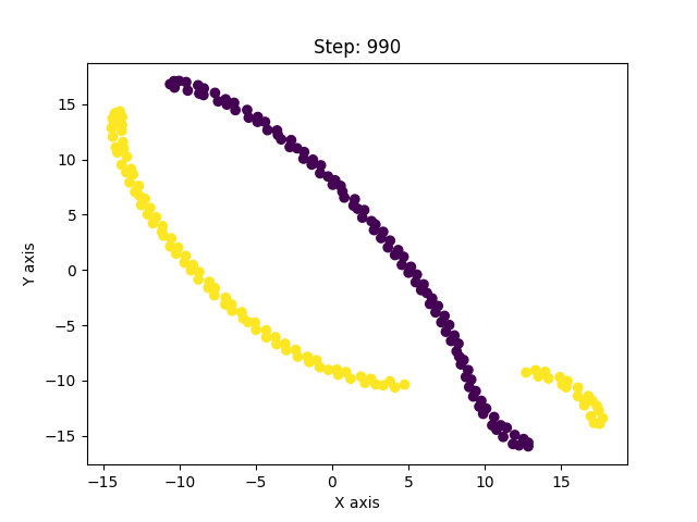
(Right) With Adam
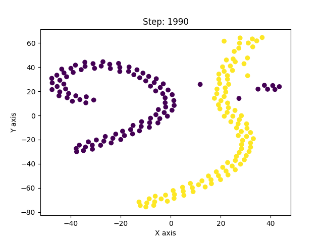
This also performs well, as can be seen from the evolution of the map points. Again, it’s worth re-iterating that this is a simple enough dataset to solve. One thing to note here is that, t-SNE is non-parametric inherently. That is, once we have the low dimensional mapping, we aren’t sure where to map any new data point that comes in next. We have to run the algorithm from scratch with this new point included to get its mapping. There was this talk by Laurens van der Maaten, the main author of the paper. They explain the concept and the algorithm really well and also go through the tips and tricks to use it in practice. During Q/A, they mentioned about exploring a parametric from of t-SNE that can be reused to compute mapping for new points without starting all over again. And to do this, I added a two layered MLP that takes the data points and outputs their 2D mapping and trained using the same optimization procedure as above. The model I added is :-
num_points = len(inp)
class SimpleMLP(nn.Module):
    def __init__(self):
        super(SimpleMLP, self).__init__()

        self.fc1 = nn.Linear(3*num_points, num_points)
        self.relu = nn.ReLU()
        self.fc2 = nn.Linear(num_points, 2*num_points)

    def forward(self, x: torch.Tensor):
        x = x.flatten()
        x = self.fc1(x)
        x = self.relu(x)
        x = self.fc2(x)
        x = x.view((num_points, 2))
        return x

model = SimpleMLP().double()
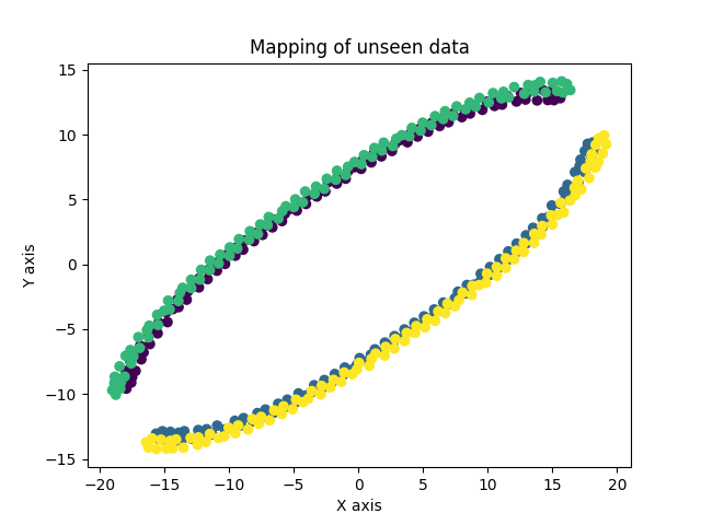
The green and yellow are the map points of an unseen region of the helices.
Under them,the purple and blue, are the map points of the original region of helices.
The results were quite good. Not only is the network able to learn the mapping well by separating the two clusters, it also is able to find mapping of unseen data points which is quite handy.
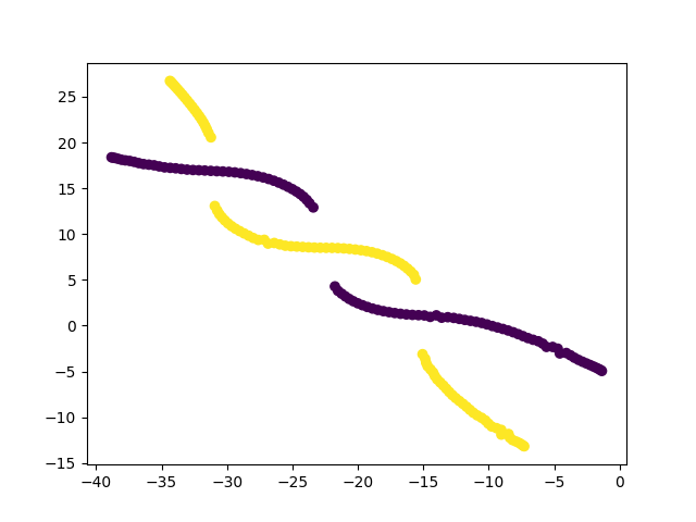
I have, so far, shown only the good solutions of the algorithm. In reality, t-SNE’s results vary from run to run even for the same parameters. And with improper optimization, it can get stuck in a local minima. Below are examples of such solutions.
This was a long post, but exploring this paper has been insightful. The paper is much more detailed and covers other concepts as well which I haven’t covered here. It led me to explore similar non-linear dimensionality techniques like Isomap, Diffusion maps, UMAP, LLE, etc. UMAP is currently considered to be the best dimensionality reduction technique as it performs better than others in many aspects. It also scales well to larger datasets, which t-SNE struggles with. The theory behind UMAP was too complicated for me to understand in its entirety but the parts that I did were quite interesting. In all of these techniques I explored, one common fundamental underlying idea is, in high-dimensional space you can only trust local regions. Which is why the concept of nearest neighbours is important. Isomap, for instance, connects nearby points together and constructs a global graph of the dataset. And, instead of taking euclidean distance, it considers the shortest path between two points in that graph as the distance between them. Only by trusting local connections, one can build an approximation to the underlying manifold. And this is where a tradeoff occurs. If the nearest neighbour radius is too small, you can imagine how the graph can be misleadingly disconnected. Conversely, if it is too large, it will connect parts of the manifold that might actually not be connected. So usually one runs these algorithms multiple times with different parameters and observes all of them to derive meaningful information. The following image from Isomap paper visually explains the concept on the swiss roll data.
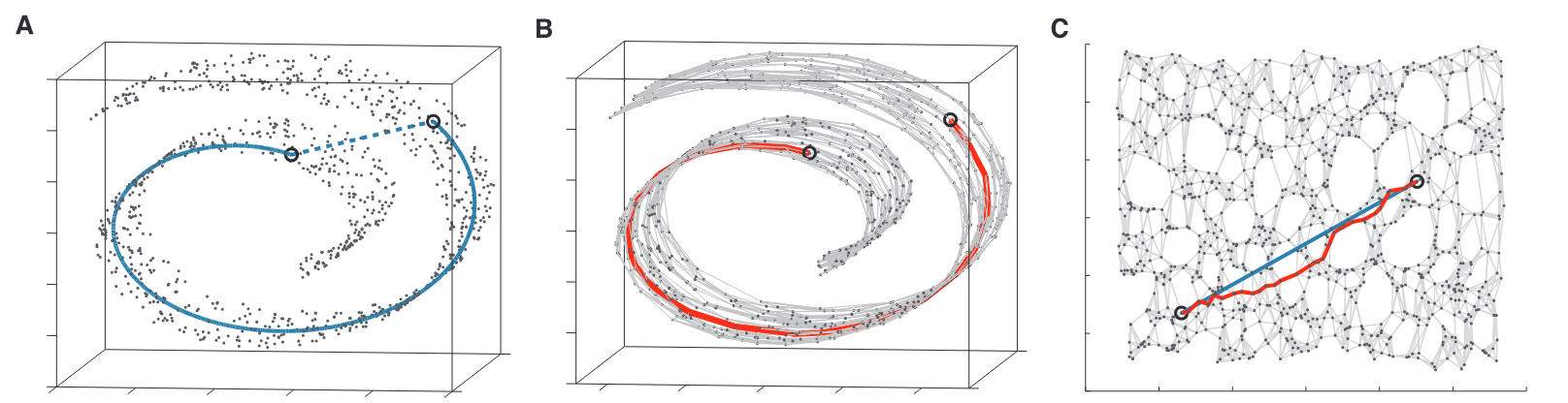
(B) A graph constructed by connecting nearby neighbours; Shortest path in the graph between the two points is higlighted
(C) An ideal 2D mapping of that data that preserves the geodesic distance
Figure taken from the Isomap paper
This was a good exercise of paper reading and implementation. Some of the papers of recent years are very well written and are the basis of many tools we are familiar with. I am keen on reading more such papers so do let me know if you have come across any such papers that made you explore and experiment on it.
The code for the experiments and other utilites used in the post is available at dibyadas/t-sne-experiments.
References:
- Laurens van der Maaten, Geoffrey Hinton Visualizing Data using t-SNE
- Deepfindr - t-distributed Stochastic Neighbor Embedding (t-SNE)
- How to Use t-SNE Effectively
- Andy Coenen, Adam Pearce Understanding UMAP
- Joshua B. Tenenbaum, Vin de Silva, John C. Langford A Global Geometric Framework for Nonlinear Dimensionality Reduction
- t-SNE implementations